Use TB2J with Wannier90
This tutorial uses cubic SrMnO\(_3\) as an example to show how to calculate the exchange parameters for the Heisenberg model starting from density functional theory. First, the Hamiltonian in the basis of Wannier functions (WF) is constructed using Wannier90. Then, TB2J is used to calculate the exchange parameters. We assume that the reader has a basic knowledge of maximally localized WFs and the Wannier90 package (see Maximally localized Wannier Functions, Wannier90).
Before beginning, you might consider to work in a subdirectory for this tutorial. Why not Work_tb2j?
The input files for the tutorial can be found inside examples/abinit-w90/SrMnO3 in your TB2J directory. Please copy abinit.in, abinit.files and the three pseudopotential files (inside the psp directory) to Work_tb2j. You also need the two files abinito_w90_down.win and abinito_w90_up.win which provide additional input for Wannier90. The names of these two files are _w90_.win with the prefix being given in the forth line of the .files file. Modify the .files file such that the entries match the location of your files.
Step 0: Find the orbitals and energy range to be used in the Wannier Function Hamiltonian.
Before we can construct the Hamiltonian in the basis of the Wannier functions, we need to determine which orbitals to include in the construction. We need to include the orbitals with energies around the Fermi energy (\(E_F\)). Since we are interested in calculating exchange parameters we need to include spin as a degree of freedom in the calculation and select the magnetic orbitals and all orbitals that overlap with them. To determine the orbitals and energy range, we calculate either the density of states or the band structure of the system. For SrMnO\(_3\) the density of states is given in the figure below.
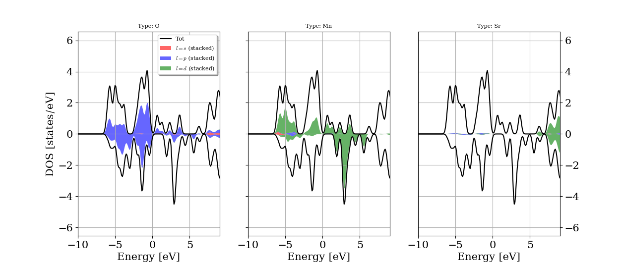
As we can see, the Mn 3d and O 2p orbitals should be included into the WF Hamiltonian. The Sr 4d orbitals are too high in energy, so we exclude them from the WF Hamiltonian.
Step 1: Construct WF Hamiltonian from DFT.
The Wannier90 code makes use of two energy windows to disentangle the bands. An outer window (the disentangle window), which contains all the required orbitals, and an inner window (the frozen window), which only contain the required orbitals, should be provided. From the DOS we find that all the Mn 3d and O 2p bands are between -10 and 10 eV, the Sr 4d bands above 6 eV, which should be excluded from the frozen window. Thus we can select the energy window (-10, 10) eV and the frozen window of (-9, 5) eV. Note that the energy defined in Wannier90 is not relative to \(E_F\), so we need to add the Fermi energy (here: 6.15 eV) to the energies. We use Mn d and O p orbitals as an initial guess for the WFs. This information can be found in the .win files
# Energy windows (Fermi energy is 6.15 eV)
dis_win_min = -3.85
dis_win_max = 16.15
dis_froz_min = 1.15
dis_froz_max = 11.15

begin projections
Mn: d
O : p
end projections
For a detailed explanation of the input variables for Wannier90 please see Wannier90. For our purpose, it is important to write out the Hamiltonian and the centers of the Wannier functions.
# write the postitions of WF
write_xyz = true

# write the WF Hamiltonian (Note for W90 version<2.1, it is hr_plot)
write_hr = true
Alternatively, the Wannier hamiltonian and the position operator can be written into one “_tb.dat” file, which can be read by TB2J since version 0.8.2
# write the WF Hamiltonian and the position operator
write_tb=ture
The following lines need to be added to the abinit input file to generate WFs.
prtwant 2    # enable wannier90
w90iniprj 2  # use projection to orbitals instead of random.
w90prtunk 0  # use 1 if you want to visualize the WF's later.
Now you can run
abinit < abinit.files > log 2> err
which generates the files below for spin up, and the same set for spin down
abinito_w90_up_hr.dat abinito_w90_up_centres.xyz abinito_w90_up.wout
The .dat file contains the Hamiltonian, the .xyz file contains the Wannier centers. The .wout file has a summary of the process of running Wannier90 and will be used to calculate the exchange parameters.
If you’re using Wannier90 version < 3.0, the spin down files are not automatically generated due to a bug. To get the files, the following command is needed:
wannier90.x abinito_w90_down
To get localized WFs can be tricky sometimes. It is necessary to check if the WFs are localized by looking at the .wout file. For example, we have
Final State
 WF centre and spread    1  (  1.904992,  1.904992,  1.904992 )     0.50185811
 WF centre and spread    2  (  1.904992,  1.904992,  1.904992 )     0.48650086
 WF centre and spread    3  (  1.904992,  1.904992,  1.904992 )     0.48650086
 WF centre and spread    4  (  1.904992,  1.904992,  1.904992 )     0.50185997
 WF centre and spread    5  (  1.904992,  1.904992,  1.904992 )     0.48650084
 WF centre and spread    6  (  1.904992,  1.904992, -0.000000 )     0.74591265
 WF centre and spread    7  (  1.904992,  1.904992,  0.000000 )     0.96557405
 WF centre and spread    8  (  1.904992,  1.904992, -0.000000 )     0.96557405
 WF centre and spread    9  ( -0.000000,  1.904992,  1.904992 )     0.96557489
 WF centre and spread   10  ( -0.000000,  1.904992,  1.904992 )     0.74589254
 WF centre and spread   11  (  0.000000,  1.904992,  1.904992 )     0.96557379
 WF centre and spread   12  (  1.904992,  0.000000,  1.904992 )     0.96557489
 WF centre and spread   13  (  1.904992, -0.000000,  1.904992 )     0.96557379
 WF centre and spread   14  (  1.904992, -0.000000,  1.904992 )     0.74589254
 Sum of centres and spreads ( 20.954915, 20.954915, 20.954915 )    10.49436382
Usually, 3d orbitals have a spread of less than 1 \(\AA\), and the O 2p orbitals have a spread of less than 2 \(\AA\).
Step 2: Run TB2J
Before running TB2J, an extra file, which contains the atomic structure, needs to be prepared. It can be either a VASP POSCAR file. (For abinit, the abinit.in file is also fine if no fancy feature is used, like use of *, or units. POSCAR files are recommended because they are simple. Note that the file extension are used to identify the format, for example, Quantum ESPRESSO input should be name with *.pwi) The supported file format are can be found on the list in: https://wiki.fysik.dtu.dk/ase/ase/io/io.html
(From version 0.6.2 this file is no more necessary as TB2J can read the atomic structures from the Wannier90 .win file). The –posfile option will still be used by default if it is specified.)
With the WF Hamiltonian generated, we can calculate the exchange parameters now. In the scripts directory inside your TB2J directory you find the wann2J.py script. Please make sure that it is executable and issue the command
wann2J.py --posfile abinit.in --efermi 6.15 --kmesh 4 4 4 --elements Mn --prefix_up abinito_w90_up --prefix_down abinito_w90_down --emin -10.0 --emax 0.0
The parameters are:
efermi: Fermi energy in eV
kmesh: k-point mesh. Default is 5 5 5
elements: the magnetic elements
prefix_up: prefix for spin up channel of the Wannier90 output
prefix_down: prefix for spin down channel of Wannier90 output.
emin: the lower limit of the electron energy. (in eV, relative to Fermi energy.)
emax: the upper limit of the electron energy. Should be zero. (Note: this parameter is no more useful will be deprecated soon).
Now we should have the files containing the J parameters in the TB2J_results directory.
TB2J_results/
├── exchange.txt
├── Multibinit
│   ├── exchange.xml
│   ├── mb.files
│   └── mb.in
├── TomASD
│   ├── exchange.exch
│   └── exchange.ucf
└── Vampire
    ├── input
    ├── vampire.mat
    └── vampire.UCF
exchange.txt: A human readable file.
Multibinit directory: the files file, input file and xml file, which can be used as templates to run spin dynamics in Multibinit.
The input for a few spin dynamics codes (Tom’s ASD, and Vampire) are also included.
Noncollinear calculation
For calculations with non-collinear spin, the –spinor option should be used. It is also necessary to specify whether in the Hamiltonian the order of the basis, either group by spin (orb1_up, orb2_up, … orb1_down, orb2_down, …) or by orbital (orb1_up, orb1_down, orb2_up, orb2_down,…), with the –groupby option (either spin or orbital). The –prefix_spinor option is used to specify the prefix of the Wannier90 outputs. Here is an example of the command:
wann2J.py --spinor --groupby spin --posfile abinit.in --efermi 6.15 --kmesh 4 4 4 --elements Mn --prefix_spinor abinito